Advance means the stock is going up and Decline means it is going down. Promotion or demotion. In the Viking, only the price of the object itself is measured, not the number of shares in an index.
The Advance Decline model is a graphical description of when the price goes up or down compared to a previous period. It does NOT tell you when to buy or sell, but is a piece of the puzzle to understand the strength or rhythm of the stock. A common perception is the rule of 3. In an upward trend, it is said that the stock goes up for three days then goes down or stays put. But is it? Look at the pictures below:
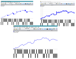
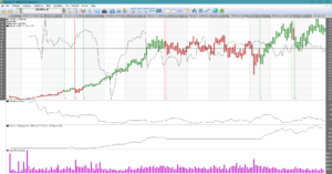
In the top chart on the left, it is presented as a Candle Stick chart. The empty squares show that the price has gone up on that day compared to the day before. It corresponds to a bar in the Advance section for each day.
Similarly when it goes down. Then the Candle Stick block is filled in and a stick appears in the Decline section below.
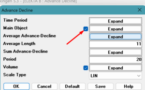
In Viking you can choose whether you want to see the price as a candle stick, line or bar chart. It is also possible to delete the course and show only the AD graph. In this case, right-click on the chart and check our main object.
Interpretation of Advance Decline
As you can see above, there are more Advance bars in an upward trend. You can quickly get a sense of whether the stock is generally going up or down. A bit like an RSI chart, the more bars at the top, the more likely the stock will soon lose momentum and go down or stand still. It will be overbought. Many bars in the Advance section mean that the stock is in a strong upward trend. If there are many bars in the Decline area, the stock is trending downwards.
Sum of Advance Decline
Total= The number of increases over a period minus the number of decreases over a period. ATTENTION! No average but a sum.
By creating a sum of the number of ups and downs, the sum is interpreted similarly to a Relative Strength Index (RSI).
When the sum of the number of rises minus falls is high, it indicates an overbought condition. When the total is low, it indicates an oversold situation. Overbought means that the price is likely to stop or fall soon. It may also mean that the rate of increase of the exchange rate is decreasing. It goes up more slowly.
On the contrary for an oversold location. When the amount is low, the price is likely to stay or go up. Or the rate of decline is slowing down.
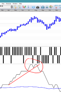
A very good interpretation, which also applies to RSI, is to look at formations. Double top, double bottom, trends, triangles, Head and shoulders. A double top at a high level indicates a very likely reversal in price.
Too short a period makes the signals too early and too long a period makes it slow. The sell signals come too late at too long a period to summarize. A value of 20 periods, day or week, is good. In the image below, it is a sum over 20 weeks. The double top indicates a reversal of the downward trend.
ACCUMULATION – DISTRIBUTION VOLUME
AD Volume
Wärtsilä gave 39 times the money with 108 weeks AD Volume average of 30 years. Wow, maybe this is a good model?
One idea with this model is that if you take the volume and mix it with a nice model like Stochastics, there should be good signals for buying and selling.
Stochastics is like a temperature gauge. When the average of the last payment is on the upper side of the bar, the stock is trending upwards. Amplifying that signal with volume should give good early signals. For a sustainable signal to provide a longer-term trend, we want the volume to be large and increasing. Applies to both buy and sell signals. Another thing about volume is that there can be an upswing. That is, if the volume is increasing and the price is flat, it is likely that the price will soon go up. This can be easily seen in an AD Volume chart. Because when last paid starts to settle on the upper half of the High-Low and the volume increases, it is easier to see it in the AD Volume chart.
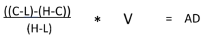
C = Close, Last L = Lowest, H = Highest, V = Volume AD=Accumulation, Distribution
If C=L, it is -(H_L)/(H-L) times the volume, i.e. -1*V. On the contrary, if C=H, then it is 1*V. The value thus varies between Volume and – Volume. Of course, the volume also varies. You could say that you get a stochastic weighted turnover. Moreover, if the volume (turnover) is high, the extreme values become more apparent.
In AD Volume you want to see if the average of AD Volume confirms the price. The average value is calculated by calculating for each period all AD Volume values and summing these values for a time. Finally, the sum is divided by the number of periods in the time period.
How good is the model?
What is the best period value? An optimization on 323 Nordic most traded stocks yielded only 49 positive results with an average of 227 days. Unfortunately, there were very different periods between stocks. In Viking, the unique period per share, index, option, etc. is saved…. when you have run an optimization in Vikingen Trading, i.e. a back testing.
Same with weekly data, scattered values, average of 167 weeks. For example, for Volvo B, the best was a 348-week average, giving a 222% increase in 43 years. A rather mediocre rise for such a long time. 233 out of 476 transactions made a profit when the computer was at its best. Fairly well, about half of them made a profit. But the results are significantly worse than Bollinger, Multimodel, MRudolph3, Kursband, BEST and Peter’s specialists.
For monthly values, there were also scattered values, with an average of 70 months. However, the chance of winning was greater. About 6 out of 10 transactions made a profit. For Volvo, 53 out of 84 transactions were profitable. 782% increase. Most people have the idea that you get richer the more you are updated. But when you run tests, it is almost always the case that weekly or monthly data is best. In other words, it is sufficient to monitor the price once a week or month. …… But it’s not as much fun and the banks don’t earn much from it.
Interpret the AD Volume charts
If the closing price is closer to the highest price than the lowest price, we have an accumulation. If instead the closing price is closer to the minimum price, we have a distribution instead. A change in a rising price trend is signaled if higher and higher peaks in the price curve do not coincide with higher and higher peaks in the mean of the AD curve.
Similarly, in a declining price trend, a reversal can be expected if the average of the AD curve’s peaks starts to reach higher and higher levels.
Price charts provide an alternative way to see if the peaks and troughs of price and volume confirm each other or not. This is done by studying whether rising peaks in the price correlate with rising peaks in the volume and vice versa.
Buy signals are given when the average curve for AD Volume crosses a bottom. Sell signals are given when the same curve has passed a peak.
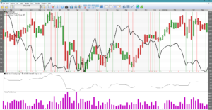
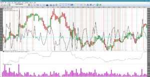
In the chart you can see that there are too many signals, especially when the price is stationary. A common problem with engineering models. You can see that it looks good when the AD Volume curve goes in the same direction as the curve. That is, the model becomes a complement to other models. The AD Volume model shows whether there is a healthy relationship between volume and last paid in relation to highest and lowest.
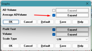
To show only the mean value of AD Volume as in the graph above, right click on the graph -> click on model parameters -> click on graphs and then just check the Mean AD Volume box. Press OK for a temporary change or Save for a permanent change.
BEST
The BEST model was created by Peter Östevik from Sweden. It was completed around 2019 after 30 years of experience. The model is a further development of Peter’s Specializer and the Optima model. Peter’s specializer is designed mostly for intraday and day rates. The BEST model is best suited with monthly data, but weekly data can also work.
But where does the name BEST come from? Simply because it is the model that works best in combination with support, resistance and trends. For several years, the model has beaten the index many times over, when combined with the weekly trend.
This is a long-term management model that increases the chances of getting rich in the long term. Feel free to browse several stocks with the model and you will probably think “I should have done that”. It is not an optimal model, but it works in practice. Works on any time series with sufficient data. Shares, funds, ETFs, indices…
How to use the model?
This is what I did when the stock market went up 6% and the BEST model made 85% in 2020. Fourteen times better than the index! All Nordic and US stocks were filtered using the BEST model.
- The condition was that shares would be in buy mode for all daily-weekly-monthly graphs. An autopilot did the job, but it is possible to filter yourself by running a signal table on day, saving those with buy signal in an item list, continuing with weekly data for the selected stocks, saving results in a new item list and running one last time with BEST and monthly data. A signal table for several shares is called a collection table in Viking.
2. Remove the shares that are close to a resistance. Those stocks are likely to stall in their rise. Also carried out a fundamental assessment of the key figures. Turnover may increase, P/S ratio below 4, P/B ratio below 3, low P/E ratio, debt ratio below 1.
3. Prioritize the stocks that have a positive trend in the monthly chart. This increases the chance that the stock will go up in the long run.
4. I built a portfolio of 15 stocks. Some were replaced when they received a sell signal.
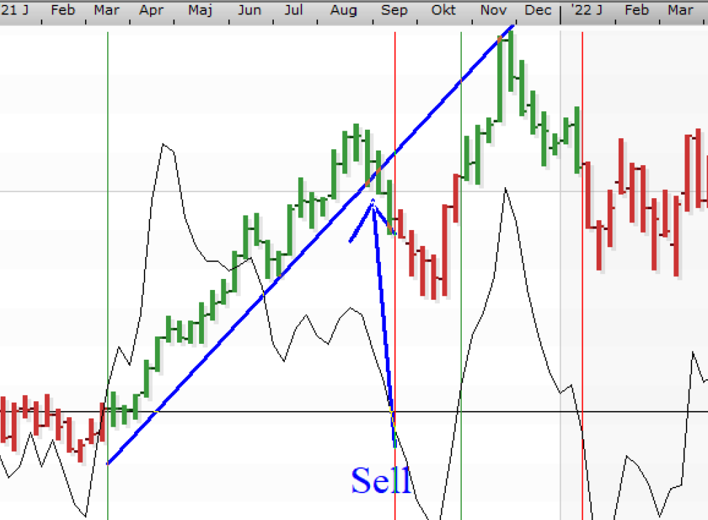
5. Shares are sold when the weekly trend is broken. Simple but effective method. Draw a line under the bottoms of the rising trend.

6. After a share has been sold, the steps above are repeated. ATTENTION! It’s NOT a buy signal every day and you shouldn’t buy!
What is included in the model ?
The model consists of several models, a so-called multi-model. Important elements are Volatility signal, RSI, average of lowest prices, average of highest prices and gap.
When prices start to diverge much more than they usually do, it is usually a good signal for further movement in that direction. The strength of the stock, as measured by the Relative Strength Index, confirms the direction of movement. We also know that various band models are good at removing unnecessary buy and sell signals, as are averaging models. If there is a strong breakout to the upside, like a gap up, it confirms the buy signal. A sudden momentum up or down also reinforces the signal.
An optimization with MONTHLY DATA gave the following approximate optimal settings:
Number of volatility periods = 4, RSI length=5, RSI average=5, Number of periods for average of lowest prices=7, Number of periods for average of highest prices=5, Number of periods for average of last paid=6, Buy percentage weight=2.5, Sell percentage weight=1.1, Buy signal multiplier=0.26, Sell signal multiplier=2.92
Beta values
Description
This model is primarily used to identify stocks that are strong or weak relative to the index.
Here, beta values are calculated, indicating the relationship between two objects, e.g.. a stock price and an index for a “Period” long period.
If the beta value is one (1.0), the price of the main object changes in the same percentage as the index. If the beta value is e.g. 1.5, this means that a (1.0) percent change in the price of the index is assumed to lead to a 1.5 percent change in the price of the main object.
Another example: If the Beta value = 2, then you can guess that the stock goes up 2% if the stock market goes up 1%.
When we talk about derivatives, the numbers are much bigger. For example, if a certificate has a beta value of 2000, the certificate goes up or down 20 times as much as the underlying object. This is called leverage 20.
Signals in the Viking
Buy if
- The beta value is greater than one AND
- The beta value is rising AND
- Index is above its average value
Sell if
- The beta value is less than -1 AND
- Index is below its average value
In addition to the standard beta value, “Beta Value Plus” and “Beta Value Minus” are also calculated for the covariance with the relative object when it is rising and falling, respectively.
Buy signals are given when “Beta valuePlus” is greater than one and rising, and when the closing price of the relative object exceeds its “MV length” long average.
Sell signals are given when the “Beta valueMinus” is greater than one and when the closing price of the relative object is below its “MV length” long average.
To give an idea of the object’s volatility, its standard deviation is also reported for the number of “Period” periods.
Good settings
Suggested values: An optimization on the most traded shares yielded:
| Average value | Period | |
| Day | 34 | 12 |
| Week | 25 | 11 |
| Month | 17 | 10 |
How good is the model?
Here is a picture of the stock Hexpol which has yielded 6 times the money with monthly data (default setting 11.11), 15 years. Of course, there are shares that perform even better, such as 350 times the money. However, the model does not work well for all objects and there are much better models that fit more generally.
For those stocks that are relatively static, the model can work well. Otherwise, the model seems to be selling too late. If the stock behaves roughly like the index, there won’t be many signals. That is, the stock market can go down slowly, which means that the model does not sell if the stock moves like the stock market. A tip is to produce a summary table for the model and rank it by Beta value. This makes it easier to trust the signals for objects with high beta values. But then you might as well use the Volatility Signal model, which gives even better signals.
Settings:
MV length = the length of the price average.
Period = the number of periods on which the beta and volatility calculations are based.
Relative objects = selection of relative objects, e.g. an index.
BOLLINGER BAND
One of the best models because it is so accurate and eliminates many unnecessary transactions. There are buy and sell signals when the price breaks out of the band and the beauty is that the width of the band adapts to how much the price moves. In times when the price fluctuates a lot, the band becomes wide and when it is calm, the band is narrow.
When the price is ‘choppy’, i.e. when volatility is high, there is a high risk of buying and selling too many times. You want to be there when it goes up and you want to sell if the price goes down a lot. But in such troubled times, it can be a good idea not to trade and wait out the storm until the market has made up its mind. That is, you only act when the band has become narrow and the price breaks out.
The width of the band can be set by choosing the length of the average and how much the band should deviate from the normal price difference, or as we say in analyst language, the standard deviation. The model calculates the normal price difference over the period and then enters a multiplier times that standard deviation, usually 2.
Interpretation
When the band is wide, you can expect the price to move in the opposite direction when the price is near a band. It becomes a support or resistance.
When the band is narrow, you can expect an eruption to occur soon. People get impatient, they wait for something to happen and eventually they can’t take it anymore and take action. Then the outbreak repeats and is amplified if many people do it at the same time. As you can see in the image below with SEB bank, there are few transactions when using weekly data. Total in this example 85 times the money in 43 years. The Viking has long data series.
Using the optimization in Viking Trading, it would be 150 times the money in the same time with the settings of 16 weeks and standard deviation 3.6.
Having good values goes a long way!
Best settings of the Bollinger Band
An optimization calculated on the most traded shares in the Nordic region, about 175 shares, gave on average the following best settings:
| Period | Means | Number of staff |
| Day | 18 | 3 |
| Week | 9 | 2 |
| Month | 4 | 1 |
The daily data was similar to the default setting, 20 and 2, while the weekly and monthly data differed significantly.
The model in detail
BollingerRSIMomentum
In the Viking there is a graph called Bollinger – RSI – Momentum. One might think that it is ONE model with all three models, a multi-model. But this is not the case. The diagram shows all three models at the same time to help you make an assessment when you see how the models interact with each other.
At the bottom of the chart is a profit curve that describes what you could have done if you traded according to the Bollinger Band signals. Below, Nvidia has given just over 50,000%, or 500 times the money in 23 years. Nvidia’s rise has been due to the popularity of Artificial Intelligenceand the need for many computer components for AI.
Bollinger band
The top of the chart shows the Bollinger band. The buy and sell signals depend solely on when the Bollinger Band is broken by the price. Very profitable model, especially with weekly data. The signals are reinforced with Momentum if Momentum rises or falls rapidly. The same applies to the RSI.
RSI, Relative Strength Index
The next model, in the middle, shows the RSI and the mean values of the RSI. A bad way to get buy and sell signals from the RSI is to watch when the RSI breaks any of its averages. This is easily proven with a simulation in Viking Trading where an optimization shows that it is a bad method. It is much better to look at the appearance of the RSI and interpret formations such as the double top and double bottom of the RSI curve. For a buy signal, it is good if the RSI rises. The sell signal in Bollinger Bands is reinforced if the RSI drops.
Momentum
Momentum is advantageously used to detect rapid changes and is popular with day traders. In Sweden, around 99% of all day traders lose money. You may be able to get in and buy at a good price, but you rarely get out with a profit. there are simply too many signals. One way to interpret Momentum is to look for when Momentum breaks its mean, but unfortunately there are often too many signals. For example, when the course is calm, there are too many signals. A better way is to look at the slope of the Momentum, also known as the derivative. A strong upward or downward sloping curve is usually a good signal to buy or sell.
Rising Momentum reinforces the buy signal in the Bollinger Band and falling Momentum reinforces the sell signal when the price breaks out of the Bollinger Band.
Momentum is also good as a warning signal, making you more alert to what is coming. If Momentum takes off, you may want to pay more attention.
The stock exchange gauge
The Exchange Meter model calculates how many items are traded in a day.
- gone up,
- have remained unchanged, or
- gone down
It also shows the percentage change of the main object. Objects included are those in the object list selected in Viking.
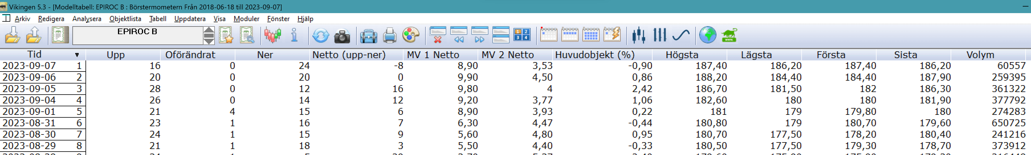
Table
Instead of Day as a period, you can choose Week or Month. That is, how many have gone up/down in a week or month. If so, click on the weekly or monthly calendar at the top of the Viking.
 Or select in the menu File -> System settings ->Models
This is a strength indicator. How strong are the items in the list? It can be a list of stocks, currencies, funds, etc. The net, i.e. the difference between the number of items going up and those going down, shows how strong that list is. It could be your portfolio. Do you have stocks that mostly go down? Then you should probably rebalance your portfolio.
An average net value is also calculated and what can you do with it? This is to get an idea of what is normal for the list. If the net deviates much from its average, it may be time to do something about it.
What can you see in the diagram?
The number of Up-Down is also shown in the RSI model and you can also see when it is overbought or oversold.
A good method is to look at the slope of the short-term average. If it starts to tilt strongly upwards, it is a sign that more items in the list will turn upwards. It’s the other way around. If the mean curves sharply downwards, more items in the list are likely to start going down.
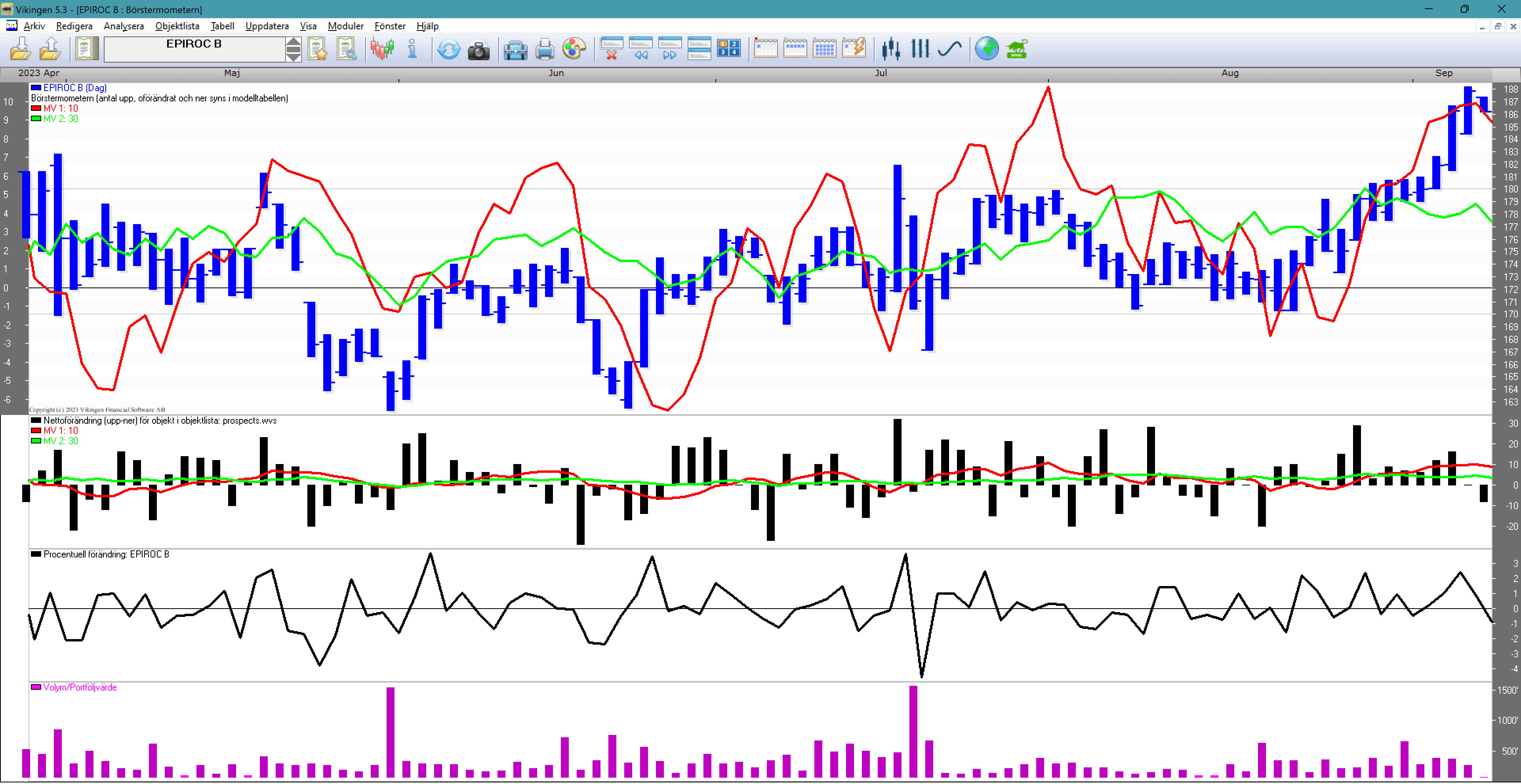
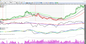
The chart in the example above is based on a list of 40 stocks. The top left-hand corner shows the number of net days included in each average (the number of up days minus the number of down days). In the example, these are averages of 10 days net and 30 days net. The short moves more than the long average. At the end of the chart you can see that the stock has done much better than the 30-day net average. That is, this stock has outperformed most of the list.
The bar chart in the middle shows whether the list is doing well or not. Many bars above zero mean up, and many bars below show that most of the list is going down.
The chart at the bottom shows the percentage rise and fall of the stock, how many percent is normal.
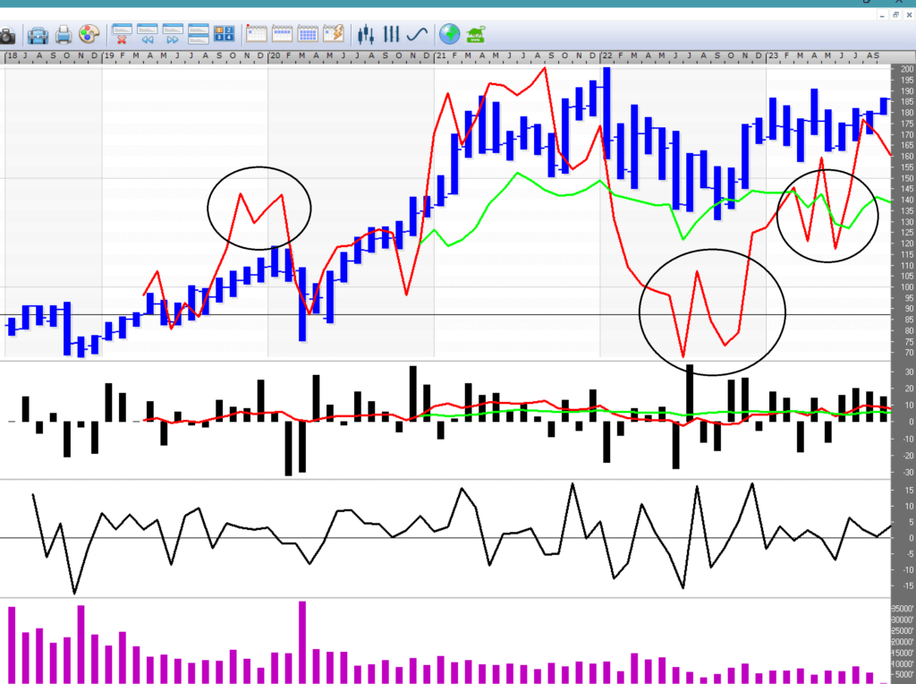
Below is the same stock but with the number of ups and downs based on months. Similar to the RSI, one can see and get signals to sell and buy by detecting double tops and double bottoms. Circled in the image.
To obtain the Stock Exchange Meter, do the following
- Select an item list and activate the Brushometer model. (Analysts -> Models -> Stock market thermometer)
- Right-click on the chart and select “Show model table”.
- The model table shows the results in numerical form.
- You can also see the percentage change of the main object.
Example with an index
Select an item list. For example, choose the OMX Stocholm 30 Index as the main item in the Viking. Then you can compare the list with the index against how many shares have gone up.
or down when the index goes up or down on a given day.
CHAIKIN
A good model for those who want to make decisions quickly. The model reacts quickly to changes and is suitable for those who monitor the price closely. Now you might think that CHAIKIN is only suitable for day trading, but the model is also suitable for trading weekly and monthly data. The model thus reacts quickly to a change in the exchange rate, whether it is per minute, day, week or month. The good news is that you can get help with selling and buying quickly. Sometimes too fast. Because when the price is essentially stationary, there are too many signals. However, it is only possible to determine afterwards whether the price was stagnant for a few days or weeks.
Probably the biggest advantage is that the risk is reduced, as you get a quick signal to sell. It also has the effect that you will sell stocks that are doing poorly, buy new ones, sell some again, buy again and finally end up in stocks that are doing well.
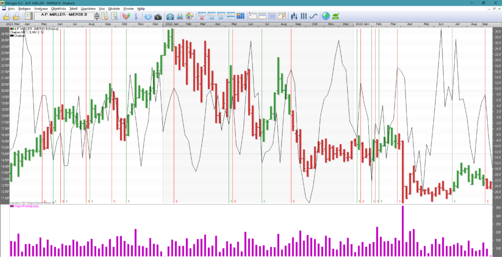
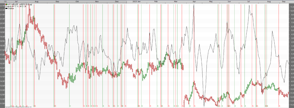
Chaikin diagram
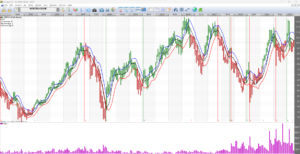
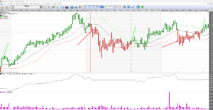
In the chart below you can see that the signals come at all extremes, both at the peaks and at the troughs. But when the price is moving sideways, it doesn’t take much to get a signal. As a user, it is difficult to know whether it is a breakout signal or just another signal. Then you can rely on volume. If there is a sharp increase in volume, you get an indication of where the price is headed. The first chart is a weekly chart, i.e. a bar shows the highest and lowest price during a week.
A red line is a sell signal and a green line is a buy signal.
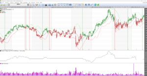
When we then switch to a daily chart with Chaikin and the same stock, there are significantly more signals. Will there be higher profits? Unfortunately, with this model it is not possible to know in advance which will be the best. Are they daily, weekly or monthly courses? If you enjoy stock market trading, you will like this model, because there is often something going on.
Good settings
On average, the settings fit for mean one = 8 and for mean two = 15. Valid for all time series, day, week, month.
The best settings differ between stocks and whether it is daily, weekly or monthly data.
Chaikin in detail
The model is a development of the ADVolume model, where AD stands for accumulation/distribution. It is used to confirm or reject a trend. It is suitable for short-term trading.
The Chaiken curve is calculated as the difference between an “MV 1 length” short average ADV volume and an “MV 2 length” long average ADV volume.
Here are two examples of applications of the Chaiken model:
1) Combine Chaiken with the curve. Weakness is indicated if the price reaches a new, higher peak, while Chaiken fails to reach its previous peak.
2) Strength is indicated if the price reaches a new, lower bottom while Chaiken does not reach below its previous bottom.
The indications are reinforced if the RSI model shows an overbought or oversold situation.
The model uses the following strategy for signals.
1) A buy signal is obtained if the Chaiken curve changes direction from falling to rising while the price curve is in a rising trend, defined in an appropriate way. For example, the trend can be defined as rising if the closing price is above an appropriately chosen long average, in the model set at 5.
2) A sell signal is obtained if the Chaiken curve changes direction from ascending to descending, while the price curve is in a descending trend, the model uses the condition that the closing price should be lower than the previous day’s closing price.
Note that the buy and sell signals here are made in the direction of the current trend, i.e. buy signals when the price trend is rising, today’s closing price above its 5-day average, and sell signals when the current price trend is falling, today’s closing price below yesterday’s.
By comparing the height of the peaks and troughs of the price curve and the Chaiken curve, one can make assumptions about the future course of the price.
The formula is as follows:
First, a ratio is calculated with the numerator as (closing price – lowest price) minus (highest price – closing price) and the denominator as (highest price – lowest price).
The ratio is then multiplied by the volume.
Settings:
MV 1 length = the length of the short average ADVolume.
MV 2 length = the length of the long average ADVolume.
Coppoch models
Signal when the sum of mean differences turns up or down. Very good results are obtained when testing backwards and saving the best settings. The problem is that the historical settings in this model are not stable. They are good historically, but my experience tells me that those settings need to be adjusted over time.
As it is a model based on averages, it is a slow model and often gives a signal too late, but still decent. The advantage of averages is that they keep the number of transactions down and give people time to act.
Below is an example with Hennes & Mauritz that has returned 5500%, i.e. 55 times the money if you traded according to the model and monitored with weekly charts. Each bar is how the course has progressed over a week. Red indicates sell and green with K, indicates buy.
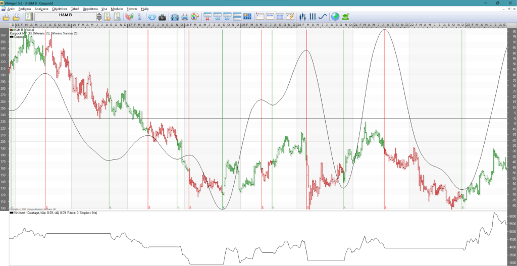
You can see in the picture that the model sometimes sells a little late, but still reasonably well.
When the price is stationary, the model changes direction frequently and there are too many signals. See below for a daily chart with Handelsbanken.
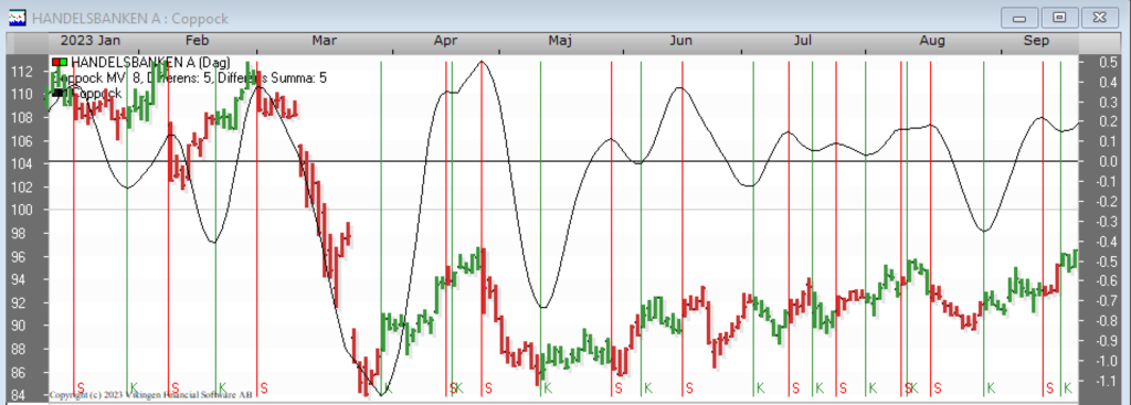
In times when prices are trending upwards and things are calm, the model works well. Then it is good to combine with other models that are faster like stochastics, volatility signal, multi-model, Peters specialists.
In general, the model seems to perform best with weekly data.
The Coppoch model in detail
The Coppock model shows the acceleration and deceleration of price developments. It also gives an indication of changes in the long-term trend.
The model is calculated as follows:
1) Calculate the moving average, A, with the length “MV length”.
2) Calculate the relative differences between mean, A, with the same mean, B, time-shifted “MV Difference” periods backwards in time.
3) Calculate the weighted sum over the “MV Difference Sum” pieces of these differences. Give the ‘oldest’ difference a weight of one and then gradually increase the weight by one.
Buy signals are given when the Coppock curve is rising.
Sell signals are given when the Coppock curve is falling.
Settings:
Mv length = the length of the price average.
MV Difference = number of periods on which the difference between the price averages is calculated.
MV Difference Total = number of differences summed up.
Good settings of the Coppoch model
With Vikingen Trading or Vikingen Maxi you can do back testing and test many combinations. The values below are the result of a test with 2.5 million combinations run on the 170 most traded shares in the Nordic region. Each share was saved with its own best optimized settings. On average, these settings were the best:
| Coppoch | |||
| Average value | Mean difference | Mean difference sum | |
| Day | 21 | 15 | 13 |
| Week | 21 | 15 | 11 |
| Month | 17 | 11 | 5 |
DCCI “Delphi Cycle Channel Index”
DCCI works best in a trend, up or down. It lets out unnecessary signals when the curls are trending.
On a daily basis, the model gives an early signal when the trend reverses. It makes a difference whether you choose daily, weekly or monthly data. For example, the result for Balder B 1999-10-12 to 2023-09-18 (24 years) was loss -62% with daily data, profit with weekly data 3200% and profit with monthly data 400%. But how do you know what to choose in advance?
Here’s a trick: Buy when the monthly model gives a buy signal and sell when the weekly trend is broken. Or if you’re just doing daily data, trade on the buy signal on the daily chart and sell when the daily trend breaks.
More examples with Delphi Channel Cyclic Index, DCCI
Too much business at a standstill. The monthly model sells and buys at the right time. Unfortunately, the sell signal comes too late sometimes, as a lot can happen in a month. Should be combined with selling when the uptrend or support is broken in the weekly model. The big advantage is that the model with monthly data does not buy or sell unnecessarily when the stock is trending up or down. The first time there is a sell signal, you do not know in advance if it will be a rectangle, but you have to follow the first sell signal and then the first buy signal in the weekly chart.
In general, it can be said that the buy signal in the monthly chart with the DCCI model is really good, it gives a good chance for a profit.
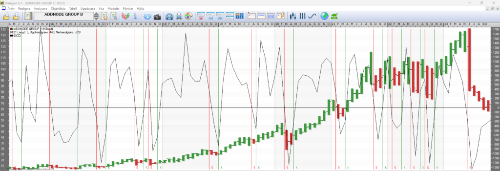
Image above DCCI with monthly data
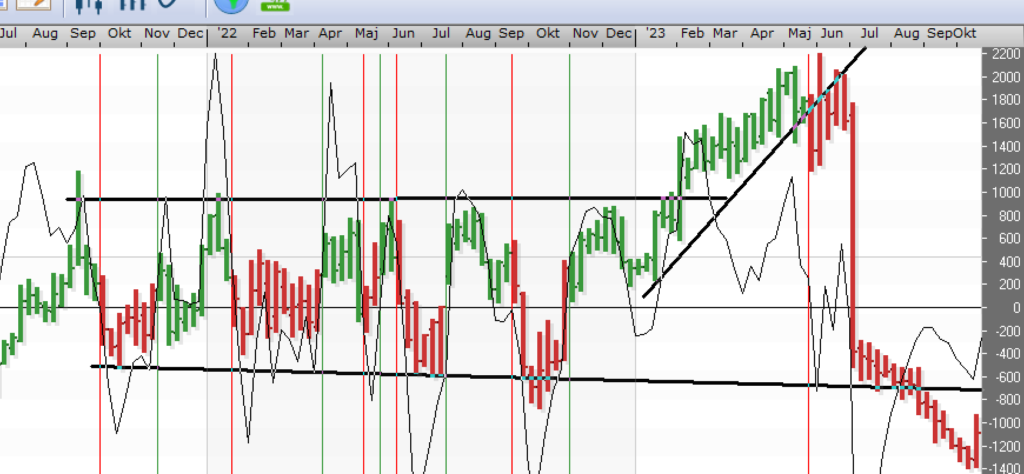
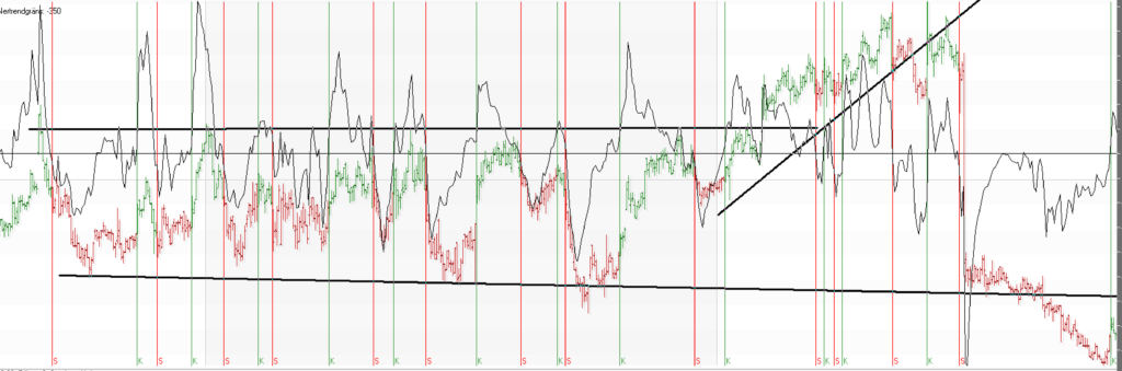
If you want something fun and interesting, you can follow the signals in the daily chart, but it is doubtful that the signals in the daily chart will be profitable.
Good settings
An optimization of the 325 most traded stocks yielded the following best settings on average:
| DCCI Length | Upward trend Limit | Downtrend Limit | |
| Day | 13 | 537 | -298 |
| Week | 9 | 503 | -296 |
| Month | 5 | 492 | -296 |
Description
DCCI is used to identify trend reversals.
High values are considered to indicate strength and low values are considered to indicate weakness.
The DCCI is calculated as follows:
1) an average, A, is taken of the closing, highest and lowest price,
2) a mean value, B, is taken on the mean value A above,
3) the difference between A and B is calculated; and
4) the difference thus obtained is divided by a number to obtain comparable figures.
Buy signals are given when the DCCI exceeds the “Up Trend Limit”, sell signals when the DCCI falls below the “Down Trend Limit”.
Settings:
DCCI length = the number of periods on which the DCCI is calculated.
Uptrend limit = level that the DCCI must exceed for a buy signal.
Downtrend limit = level below which the DCCI must fall for a sell signal.
Background
The first version of the Vikingen stock exchange program was created by Delphi Economics, which started in Uppsala and continued in Stockholm. Hence the word ‘Delphi’.