Chaikin Oscillator
Description:
In the Viking called Chaikin
Inspired by the work of his predecessors (Joe Granville and Larry Williams), Mark Chaikin developed a new volume model.
The Chaikin Oscillator model uses a moving average based on the Accumulation/Distribution model.
I’ll let Mark Chaikin himself tell the story. The translation is by me but the words are written by Mr. Chaikin himself.
“Technical analysis of both indices and individual stocks, must include volume in the studies to give the technician a true picture of the internal dynamics of a given market. Volume analysis helps to identify internal strength and weakness, which exist in the protection of the course development. Very often, volume divergences against price movements are the only clues we get, that an important trend reversal is imminent. While volume has always been mentioned by engineers and found to be important, not much effective work has been done to develop volume models until Joe Granville and Larry Williams began to look at volume versus rate, in the latter half of the 1960s, in a more creative way.
For many years, it was accepted that volume usually rose and fell together and when this relationship changed, the price development would be examined for a possible trend reversal. The Granville OBV concept, which sees the total volume on an up day as accumulation and the total volume on a down day as distribution, is a decent concept, but far too simple to be of real value. The reason for this is that it generates far too many peaks and troughs, both short-term and medium-term, as OBV confirms extreme prices. However, when an OBV line gives a divergence signal towards the price extreme, it can be a valuable technical signal that usually reverses the price trend.
Larry Williams took the OBV concept and improved it. To determine whether there was accumulation or distribution in the market or in an individual stock on a given day, Granville compared the closing price to the previous closing price, with Williams comparing the closing price to the opening price. He (Williams) created a so-called Cumulative line by adding a percentage of the total volume to the line if the closing price was higher than the opening price and subtracting a percentage of the total volume if the closing price was lower than the opening price. The accumulation/distribution line was significantly improved over the classic OBV approach to volume divergence.
Williams then went a step further, when he analyzed the Dow Jones Industrials, by creating an oscillator of the Accumulation/Distribution line and still got better buy and sell signals. In the early 1970s, the opening price was removed from newspapers and Williams’ formula became difficult to use without a series of daily phone calls to a stockbroker who had access to the opening prices. Because of this gap, I created the Chaikin oscillator model by replacing the Williams opening price with the average price for the day and also took the concept a step further by applying the oscillator to stocks and commodities. The Chaikin model is an excellent model for generating buy and sell signals when its movements are compared with price movements. I am convinced that it is a significant improvement on the work that preceded it.
The purpose of my oscillator is threefold.
The first rule is that if a stock or index closes above its midpoint for the day (defined as [high + low] / 2), then it was a day of accumulation. The closer a stock or index closes to its high, the more accumulation there was that day. Conversely, if a stock or index closes below its midpoint for the day, it was a distribution day. The closer a stock closes to its closing price, the more distribution there was that day.
The second premise is that a healthy rally is accompanied by an increase in volume and strong volume accumulation. Since volume is the fuel for a rally, it follows that lagging volume during a rally is a sign that there is less fuel available to propel the stock higher.
Conversely, declines are accompanied by lower volume but end with a panic-driven liquidation by institutional investors. Therefore, we look for an increase in volume followed by lower lows on reduced volume with some accumulation before a valid bottom can form.
The third proposition is, by using the Chaikin model, you can monitor the volume flow in and out of a market. By comparing this flow with price developments, one can identify peaks and troughs, both in the short and medium term.
As no technical model works all the time, I suggest using the model together with other technical models to avoid problems. I favor the use of a price range around a 21 day moving average and an overbought/oversold model along with the Chaikin model for best short and medium technical signals.
The main signal generated by Chaikin occurs when the price reaches a new high or a new low in a rebound, especially at an overbought or oversold level, and the model fails to exceed previous extremes and then reverses direction.
1. Signals in the direction of the trend are more reliable than those that go against the trend.
2. A confirmed high or low does not imply that the price will continue moving in that direction. I consider it a non-event.
A second way to use the Chaikin model is to see the directional change in the model as a buy or sell signal, but only in the direction of the trend. For example; If a stock is above its 90 day moving average in an uptrend and an upward reversal of the oscillator while in negative territory, a buy signal is generated only if the stock is above its 90 day moving average — not below.
A downward reversal, while the oscillator is in positive territory (above 0) would generate a sell signal if the stock is below its 90-day moving average.
Chaikin is calculated by subtracting a 10-day exponential moving average on the Accumulation/Distribution line from a 3-day exponential moving average on the Accumulation/Distribution line.
Interpretation:
Above, I have translated Mark Chaikin’s own text and included an image in which he illustrates what it is supposed to look like. This is his own interpretation.
Chaikin is simply MACD applied to the A/D line.
In the Viking, it might look like this:
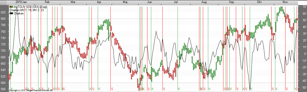
Since we have learned not to rely on a single model and we have now identified a divergence, we use other models to confirm this and, if necessary, provide us with sell or buy signals.
It is necessary to choose models that complement each other and avoid using models that show the same things. It is therefore superfluous to produce Momentum and or MACD together with Chaikin. They are all based on the same things. Stochastic, CCI and RSI are all ‘banding’ (momentum) models that are good at showing overbought and oversold positions. They are a good complement to Chaikin.
Here I show Chaikin and RSI on the same time scale. RSI provides confirmation and the sell signal while Chaikin provides the early warning that something is happening. Of course, we also seek confirmation in the volume and formations we draw in our diagrams.
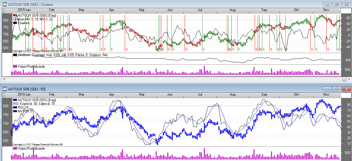
A good combination for Chaikin could be the following:
The Chaikin Model – A non-trend-following volume model used to identify buying and selling pressure.
RSI – A momentum model used to identify potential overbought and oversold conditions.
Moving Average – A trend-following model for identifying the underlying trend in a stock.
Price Relative – A comparative model for identifying the strength of a stock relative to an industry index or the OMX, for example.
These four models have very little in common and complement each other very well.
Passus:
The Chaikin model, unlike a momentum model, is not affected by day-to-day price changes. Instead, it focuses on the position of the closing price in relation to a period. This is the strength of the Chaikin model but also its weakness. Pga. because it does not reflect the day-to-day exchange rate change, sometimes large gaps are not reflected in the model. Sometimes it can even move in the opposite direction from ‘Gappet’ and give a misleading picture.
As long as the Chaikin curve is above the 0 line, it is bullish.
The Chaikin model is suitable for short trading and should definitely not be used alone.
Source: Greger
CHAIKIN
A good model for those who want to make decisions quickly. The model reacts quickly to changes and is suitable for those who monitor the price closely. Now you might think that CHAIKIN is only suitable for day trading, but the model is also suitable for trading weekly and monthly data. The model thus reacts quickly to a change in the exchange rate, whether it is per minute, day, week or month. The good news is that you can get help with selling and buying quickly. Sometimes too fast. Because when the price is essentially stationary, there are too many signals. However, it is only possible to determine afterwards whether the price was stagnant for a few days or weeks.
Probably the biggest advantage is that the risk is reduced, as you get a quick signal to sell. It also has the effect that you will sell stocks that are doing poorly, buy new ones, sell some again, buy again and finally end up in stocks that are doing well.
Chaikin diagram
In the chart below you can see that the signals come at all extremes, both at the peaks and at the troughs. But when the price is moving sideways, it doesn’t take much to get a signal. As a user, it is difficult to know whether it is a breakout signal or just another signal. Then you can rely on volume. If there is a sharp increase in volume, you get an indication of where the price is headed. The first chart is a weekly chart, i.e. a bar shows the highest and lowest price during a week.
A red line is a sell signal and a green line is a buy signal.
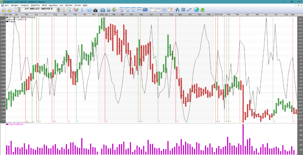
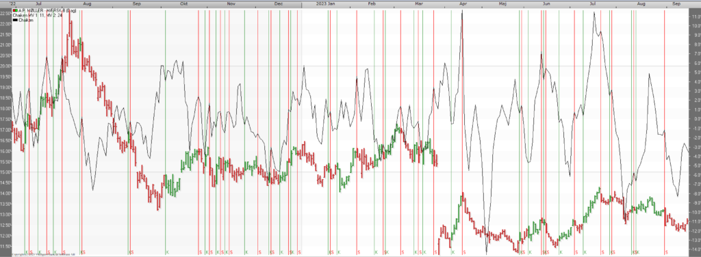
When we then switch to a daily chart with Chaikin and the same stock, there are significantly more signals. Will there be higher profits? Unfortunately, with this model it is not possible to know in advance which will be the best. Are they daily, weekly or monthly courses? If you enjoy stock market trading, you will like this model, because there is often something going on.
Good settings
On average, the settings fit for mean one = 8 and for mean two = 15. Valid for all time series, day, week, month.
The best settings differ between stocks and whether it is daily, weekly or monthly data.
Chaikin in detail
The model is a development of the ADVolume model, where AD stands for accumulation/distribution. It is used to confirm or reject a trend. It is suitable for short-term trading.
The Chaiken curve is calculated as the difference between an “MV 1 length” short average ADV volume and an “MV 2 length” long average ADV volume.
Here are two examples of applications of the Chaiken model:
1) Combine Chaiken with the curve. Weakness is indicated if the price reaches a new, higher peak, while Chaiken fails to reach its previous peak.
2) Strength is indicated if the price reaches a new, lower bottom while Chaiken does not reach below its previous bottom.
The indications are reinforced if the RSI model shows an overbought or oversold situation.
The model uses the following strategy for signals.
1) A buy signal is obtained if the Chaiken curve changes direction from falling to rising while the price curve is in a rising trend, defined in an appropriate way. For example, the trend can be defined as rising if the closing price is above an appropriately chosen long average, in the model set at 5.
2) A sell signal is obtained if the Chaiken curve changes direction from ascending to descending, while the price curve is in a descending trend, the model uses the condition that the closing price should be lower than the previous day’s closing price.
Note that the buy and sell signals here are made in the direction of the current trend, i.e. buy signals when the price trend is rising, today’s closing price above its 5-day average, and sell signals when the current price trend is falling, today’s closing price below yesterday’s.
By comparing the height of the peaks and troughs of the price curve and the Chaiken curve, one can make assumptions about the future course of the price.
The formula is as follows:
First, a ratio is calculated with the numerator as (closing price – lowest price) minus (highest price – closing price) and the denominator as (highest price – lowest price).
The ratio is then multiplied by the volume.
Settings:
MV 1 length = the length of the short average ADVolume.
MV 2 length = the length of the long average ADVolume.


